February 17, 2022
\(
\newcommand{\etal}{\textit{et al.}}
\newcommand{\afv}{A\(^\ast\)FV}
\newcommand{\calR}{\mathcal{R}}
\newcommand{\bigO}{\mathcal{O}}
\newcommand{\bfc}{\mathbf{c}}
\newcommand{\relu}{\mathsf{ReLU}}
\def\code#1{\texttt{#1}}
\def \a {\alpha}
\def \b {\beta}
\def \d {\delta}
\def \e {\epsilon}
\def \g {\gamma}
\def \k {\kappa}
\def \lam {\lambda}
\def \s {\sigma}
\def \t {\tau}
\def \ph{\phi}
\def \v {\nu}
\def \w {\omega}
\def \ro {\varrho}
\def \vare {\varepsilon}
\def \z {\zeta}
\def \F {{\mathbb F}}
\def \Z {{\mathbb Z}}
\def \R {{\mathbb R}}
\def \deg {{\rm deg}}
\def \supp {{\rm supp}}
\def \l {\ell}
\def \Aut {{\rm Aut}}
\def \Gal {{\rm Gal}}
\def \A {{\mathcal A}}
\def \G {{\mathcal G}}
\def \H {{\mathcal H}}
\def \P {{\mathcal P}}
\def \C {{\mathcal C}}
\)
1. Introduction
CKKS, a.k.a. Homomorphic Encryption for Arithmetic of Approximate Numbers
(HEAAN), was proposed to offer homomorphic computation on real numbers.
The main idea is to consider the noise, a.k.a. error $e$, which is introduced
in Ring-Learning with Errors (Ring-LWE) based FHE schemes for security
purposes, as part of the message $\mu$ (which we call here payload) we want
to encrypt. The payload and the noise are combined to generate the plaintext
($\mu+e$) that we encrypt.
Thus, the encryption procedure takes in $(\mu + e)$ as input and generates a ciphertext that encrypts an approximate value of our payload. The rationale behind this is that if the noise is much lower in magnitude compared to the payload, it might not have a noticeable effect on the payload or results of computing over the payload. In fact, even in the normal context without considering encryption, computers use fixed-point or floating-point representations to handle real data. Some real data cannot be represented exactly using these systems, and all we can do is to approximate them with a predefined precision via standard truncation or rounding procedures. This approximation results in errors that can accumulate and expand during computation. But for most realistic scenarios, the errors are not much significant and the final result is therefore satisfactory. Therefore, we sort of can think of the RLWE error in the encrypted domain as truncation or rounding error in the clear domain.
Similar to other FHE schemes, in CKKS, as we compute on ciphertexts, the plaintext (which includes the payload and the error) magnitude grows. If we add two ciphertexts, the growth is limited, but, if we multiply them, the growth is rather higher. Take an example $\mu_1 = 2.75$ and $\mu_2 = 3.17$. The product of $\mu_1 \cdot \mu_2 = 8.7175$. Clearly, the number of digits in the product has doubled. Assuming we fixed the precision at two decimal digits, the product can be scaled down by 100 to produce $\hat{\mu}^{\times} = 8.71$ (if we use truncation) or $\tilde{\mu}^{\times} = 8.72$ (if we use rounding). Generally speaking, both values are good approximates of the exact value of the product adequate for most realistic scenarios. In this rather simplified example the precision is only 2 decimal digits, in IEEE-754 single- and double-precision standards, the precision is fixed at 7 and 15 digits, respectively, providing much more accurate results.
While scaling down is a trivial procedure in the clear domain, it is generally quite expensive in the encrypted domain. Earlier solutions suggest approximating the rounding function as a polynomial for extracting and removing lower digits of encrypted values [HS15, CH18]. We know that FHE is ideally well suited for evaluating polynomials on encrypted data making this approach sensible and straightforward to implement. Unfortunately, this approach is computationally expensive and may not be practical for general scenarios due to the large degree of these polynomials. This, however, has entirely changed after CKKS.
At the heart of the CKKS scheme is a mechanism, called $\textsf{RESCALE}$, that is used to reduce the magnitude of the plaintext (payload and noise). This procedure can be used to simulate the truncation procedure very efficiently. CKKS employed the commonly known FHE procedure $\textsf{MODSWITCH}$ (short for modulus switching) that is mostly used in the BGV scheme, as described in our previous article, to implement this rescaling functionality. In fact, one shall soon notice the great similarity between the two schemes.
CKKS decryption generates an approximate value of the payload $(\mu + e)$ with adequate precision. Only if the magnitude of the error is much smaller than that of the payload, this would be acceptable. Fortunately, this is generally the case - given that the scheme is parameterized wisely - since the noise can be controlled as will be described later.
CKKS $\textsf{RESCALE}$ provides a natural way to compute on encrypted real numbers unlike other FHE schemes (such as Fan-Vercauteren (FV) [FV12] or Brakerski-Gentry-Vaikuntanathan (BGV) [BGV14]) that compute naturally on integers. It should be remarked that one can perform homomorphic computation on encrypted real numbers using BFV and BGV, but that requires sophisticated (and generally inefficient) encoding procedures [CSVW16]. Moreover, scaling down the results during computation is rather difficult.
To get an idea of how CKKS works, Figure 1 can be of aid. The figure shows the ciphertext structure of BGV and CKKS. The ciphertext in BGV and CKKS (and even for BFV) is typically a pair of polynomials. One polynomial contains the payload information while the other is used for decryption. The coefficients of these polynomials are bounded by the integer $q$, known as the ciphertext coefficient modulus, that is, they can take any value between $0$ and $q-1$. Without loss of generality and for ease of illustration, suppose the polynomials are of degree $0$. In Figure 1, we show the polynomial that contains the payload information in both BGV and CKKS schemes.
1.1 BGV Ciphertext Structure
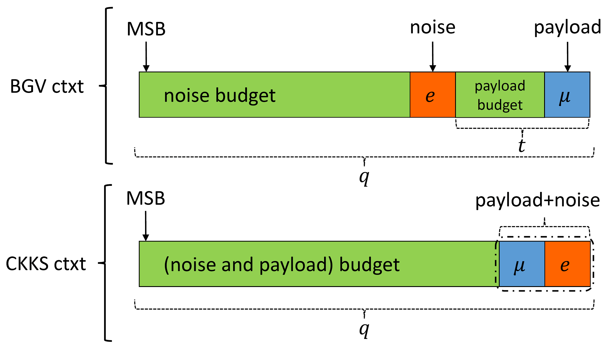
Let's first study the BGV ciphertext structure. It is useful to keep this analogy
in mind and think of the ciphertext as a bounded space. The green-colored areas
are the open space an entity may reside in. The space in our ciphertext is
bounded by the value of $q$. Two main entities are of particular interest, the
payload $\mu$ and the noise $e$. In BGV, these two components are separated and
should not interact at any stage of the computation, otherwise, the payload will
be lost. The separation is simply done by scaling the noise component $e$ by $t$
during encryption. This will shift the error to the left by $t$ as depicted in
Figure 1 (BGV ctxt). The payload can freely move in the space bounded by $t$,
i.e., taking any value between $0$ and $t-1$. This should be maintained during
homomorphic computation as well. The noise component $e$ is free to move in the
space bounded by $t$ to $q-1$ (actually less than that but let's not get into
details to keep the illustration simple). As long as the error or the payload
resides in their respective space, decryption works and the expected payload or
computed results can be retained with zero loss in precision.
1.2 CKKS Ciphertext Structure
The ciphertext in the CKKS scheme has a slightly different structure. Firstly,
the two main components $\mu$ and $e$ are combined to form one single entity.
The noise is part of the payload. As a matter of fact, there is no way of
separating these two components (to their exact values) after encryption.
This larger entity can now move freely in the space bounded by $q$. One might
legitimately wonder that combining $\mu$ and $e$ might distort or corrupt the
payload, especially if the payload is of small magnitude (same order of $e$).
This is a valid concern and addressing it is quite simple, CKKS scales the
payload by a parameter, known as the scale factor $\Delta$. This will move
the most significant bits of the payload to the left farther from $e$. The
assumption is that the least significant bits of $\mu$, which will be distorted
by adding $e$, are not of much significance which happens to be true in practice.
To help you see why this is the case, let's work out the following example.
Example 1.1. Let $\mu = \pi = 3.14159265358979323846 \ldots$, $e = 20$ and $\Delta = 10^6$. Assume we are using truncation for trimming down the least significant digits after scaling. We have: $\Delta \cdot \mu + e = 3141592+20 = 3141612$, which is still a good approximation of the scaled payload. If we want to retrieve the original payload, we can simply divide by the scale factor. Thus we have, $3141612/10^6=3.141612$ which is, generally speaking, still a good approximation of $\pi$. We could get a better approximation if we used a larger $\Delta$.
Before we delve further into describing CKKS primitives more concretely, it would be good to brush up on fixed-point arithmetic since what CKKS does, is actually simulating fixed-point arithmetic in the encrypted domain. We refer the reader to Appendix A for an overview of fixed-point arithmetic.
2. Plaintext and Ciphertext Spaces
In CKKS, the plaintext and ciphertext spaces are almost the same. They
include elements of the polynomial ring $R_q = \Z_q[x]/f(x)$, where $q$
is an integer called the coefficient modulus and $f(x)$ is a polynomial
known as the polynomial modulus. Elements of $R_q$ are polynomials with
integer coefficients bounded by $q$. Their degrees are also bounded by
the degree of $f(x)$. The most common choice of $f(x)$ in the literature
is $f(x)=x^n+1$ with $n$ (known as the ring dimension) being a power of
2 number. The difference between CKKS plaintext and ciphertext instances
is the number of ring elements they contain. An instance of CKKS plaintext
includes one ring element (polynomial) whereas an instance of CKKS
ciphertext includes at least 2 ring elements.
The previous paragraph might be thought of as contradicting to what CKKS was originally proposed for, i.e., computing on encrypted real numbers since the plaintext is a polynomial with integer coefficients. The key idea to note is that, CKKS proposes new encoding and decoding ($\textsf{codec}$) techniques, that will be described later, to map a vector of real numbers (more precisely complex numbers) into the plaintext space and vice versa. As we mentioned previously, CKKS simulates fixed-point arithmetic operations which can be done on integral operands via integer operations.
3. Plaintext Encoding and Decoding
Another main contribution of the CKKS work [CKKS17] is a new $\textsf{codec}$
method that maps a vector of complex numbers into a single plaintext object
and vice versa. Encoding works as follows, given an $\frac{n}{2}$-vector of
complex numbers $z \in \mathbb{C}^{\frac{n}{2}}$, return a single plaintext
element $a \in R$. Decoding does reverse encoding by taking a plaintext
element and returning a vector of complex numbers.
This is done using Equation \ref{eq:ckks:codec}. The map $\pi$ is the complex
canonical embedding which is a variant of the Fourier transform.
\begin{equation}\label{eq:ckks:codec}
\begin{split}
\textsf{ENCODE}(z, \Delta) &= \lfloor \Delta \cdot \pi^{-1}(z) \rceil\\
\textsf{DECODE}(a, \Delta) &= \pi(\frac{1}{\Delta}\cdot a)
\end{split}
\end{equation}
It should be clear by now the connection between the CKKS $\textsf{codec}$ scheme and fixed-point representation. While we encode the input payload, scaling is done by multiplying by $\Delta$ and removal of least significant fractional parts is done via rounding. In decoding, we reverse this procedure. Multiplying by $\Delta$ and rounding in encoding and division by $\Delta$ in decoding are similar to what we did in fixed-point encoding in Equation \ref{eq:conv:real:to:fixed}.
4. Parameters
So far, we came across the parameters $n$, $q$ and $\Delta$. CKKS uses the following
additional Ring-LWE-specific distributions in its instantiation:
Regarding the choice of the parameters $(q, n)$, the same discussion we made in the BFV article also applies here. One thing to note is that $q$ should be large enough to support the desired multiplicative depth of the computed circuit. Given the value of $q$ is fixed, $n$ is determined to provide a sufficient security level. For this purpose, an RLWE hardness estimator can be used [APS15].
We remark that, unlike the BFV scheme we described in our first article, CKKS is a scale-variant scheme. This means that at each level, there is a different coefficient modulus. Remember, as we perform homomorphic multiplication, the ciphertext is scaled down by $\Delta$. This results in reducing the size of $q$ by $\Delta$ and we end up in a ring whose coefficient modulus is $q'=\frac{q}{\Delta}$. Hence, hereafter, we refer to the coefficient modulus at level $l$ by $q_l$, where $1 \leq l \leq L$, and $L$ is the level of a freshly encrypted ciphertext. Therefore, our ciphertext coefficients are related to each other by: \begin{equation} q_L > q_{L-1} > \ldots > q_1 \end{equation}
5. Key Generation
This procedure is quite similar to the Key Generation procedure in BFV. We sample
the secret key $\textsf{SK}$ an element from $R_2$, i.e., a polynomial of degree $n$
with coefficients in $\{-1,0,+1\}$.
The public key $\textsf{PK}$ is a pair of polynomials $(\textsf{PK}_1, \textsf{PK}_2)$
calculated as follows:
\begin{align}
\textsf{PK}_1 &= [-a\cdot \textsf{SK} + e]_{q_L} \\ \textsf{PK}_2 &= a \xleftarrow{\mathcal{U}} R_{q_L}
\end{align}
Thus, $a$ is a random polynomial sampled uniformly from $R_{q_L}$, and $e$ is a
random error polynomial sampled from $\mathcal{X}$. Recall that the notation
$[\cdot]_{q_L}$ implies that polynomial arithmetic should be done modulo $q_L$.
Note that as $\textsf{PK}_2$ is in $\R_{q_L}$, polynomial arithmetic should also
be performed modulo the ring polynomial modulus $(x^n+1)$.
6. Encryption and Decryption
To encrypt a plaintext message $\textsf{M}$ in $R$ (which is an encoding of the
input payload vector). We generate 3 small random polynomials $u$ from $R_2$
and $e_1$ and $e_2$ from $\mathcal{X}$ and return the ciphertext
$\textsf{C} = (\textsf{C}_1,\textsf{C}_2)$ in $R_{q_l}^2$ as follows:
\begin{align}\label{eq:encrypt}
\textsf{C}_1 &= [\textsf{PK}_1\cdot u + e_1 + \textsf{M}]_{q_l}\\
\textsf{C}_2 &= [\textsf{PK}_2\cdot u + e_2]_{q_l} \nonumber
\end{align}
The only difference between encryption in CKKS from that in BFV is that we do
not scale $\textsf{M}$ by a scalar. Note that we can encrypt and generate a
ciphertext at any level $l$.
Decryption is performed by evaluating the input ciphertext in level $l$ on the secret key to generate an approximate value of the plaintext message: \begin{equation} \label{eq:decryption} \hat{\textsf{M}} = [\textsf{C}_1 + \textsf{C}_2\cdot \textsf{SK}]_{q_l} \end{equation} We leave the proof of why decryption works to the reader as an exercise. You might want to review our BFV article for some help on how to tackle this challenge.
7. Homomorphic Evaluation
We move now to describe how homomorphic operations are performed in CKKS.
We are interested in two operations, homomorphic addition and homomorphic
multiplication. The former is quite similar to that of BFV. The latter needs
to be followed by rescaling to maintain the precision of computation unchanged.
7.1 EvalAdd
Similar to BFV $\textsf{EvalAdd}$, we just add the corresponding polynomials
in the input ciphertexts as shown in Equation \eqref{eq:homo:add}. Note
that the input ciphertexts are assumed to be on the same level with the same
scale. If that is not the case, we need to scale down the ciphertext at the
higher level to match the scale and level of the other ciphertext.
\begin{equation}\label{eq:homo:add}
\textsf{EvalAdd}(\textsf{C}^{(1)}, \textsf{C}^{(2)}) = ([\textsf{C}^{(1)}_1 + \textsf{C}^{(2)}_1]_{q_l}, [\textsf{C}^{(1)}_2 + \textsf{C}^{(2)}_2]_{q_l}) = ( \textsf{C}^{(3)}_1, \textsf{C}^{(3)}_2) = \textsf{C}^{(3)}
\end{equation}
7.2 EvalMult
Again, this procedure proceeds similar to $\textsf{EvalMult}$ in BFV. The
derivation is also similar to what we did in BFV and we leave it to the
reader as an exercise. We only show how to compute $\textsf{EvalMult}$ on
two ciphertexts as follows:
\begin{equation}
\begin{split}
\textsf{EvalMult}(C^{(1)}, C^{(2)}) = \bigg( &[\textsf{C}^{(1)}_1\cdot\textsf{C}^{(2)}_1]_{q_l}, [\textsf{C}^{(1)}_1 \cdot \textsf{C}^{(2)}_2 + \textsf{C}^{(1)}_2 \cdot \textsf{C}^{(2)}_1 ]_{q_l}, \\& [\textsf{C}^{(1)}_2 \cdot \textsf{C}^{(2)}_2]_{q_l} \bigg) = ( \textsf{C}^{(3)}_1, \textsf{C}^{(3)}_2, \textsf{C}^{(3)}_3) = \textsf{C}^{(3)}
\end{split}
\end{equation}
8. RESCALE
This procedure does not exist in the scale-invariant version of BFV we discussed
in our
first article.
It is worth mentioning that BFV can also be instantiated as a scale-variant scheme.
In that case, a procedure called $\textsf{MODSWITCH}$ can be used to switch between
the ciphertext coefficient moduli. CKKS adapted the $\textsf{MODSWITCH}$ procedure and
called it $\textsf{RESCALE}$. Mathematically, they are the same, but they serve two
different purposes. The main purpose of using it in CKKS is typically to reduce the
scale factor after multiplication to match that of the input ciphertexts. The procedure
is quite simple and computationally efficient, it takes a ciphertext
$\textsf{C} \in R_{q_l}^2$ and scales it down by $\Delta$ to generate an equivalent
ciphertext $\hat{\textsf{C}} \in R_{q_{l-1}}^2$ encrypting the same plaintext but
with reduced scale factor and reduced noise. This procedure simulates the rescaling
step ($\frac{1}{2^f}$) in Equation \ref{eq:FPMul} but in the encrypted domain.
\begin{equation}\label{eq:rescale}
\textsf{RESCALE}(\textsf{C}, \Delta) = \frac{1}{\Delta}\cdot [\textsf{C}_1, \textsf{C}_2]_{q_l} = [\hat{\textsf{C}}]_{q_{l-1}}
\end{equation}
9. Intuition of Multiplication in CKKS
As we said previously, CKKS simulates fixed-point arithmetic in the encrypted domain.
Figures 2 and 3 can help in understanding how this can be realized. First, we
study how homomorphic multiplication works in BGV. Again, we assume our ciphertext
has 2 polynomials, each with a single coefficient. Also, we only focus on the
polynomial that contains the payload.
As shown in Figure 2, multiplication causes both components (payload) and noise to grow in magnitude. The multiplication result is contained within the space bounded by $t$, i.e., in the lower bits of the coefficient. The noise in the product grows similarly and takes some space from the noise budget. As mentioned previously, as long as the payload and noise are separate, decryption works successfully and the payload can be retrieved without errors. To obtain more intuition about the product ciphertext structure, let's work out the following algebraic equation: \begin{equation}\label{eq:bgv:mult:structure} \begin{split} \mu_1 \cdot \mu_2 + e'_{\times} &= (t e_1+\mu_1) \cdot (t e_2+\mu_2)\\ &= t^2 e_1 e_2 + t(e_1 \mu_2 + e_2 \mu_1) + \mu_1\mu_2 \end{split} \end{equation} To reduce the noise growth after multiplication, BGV includes a method called $\textsf{MODSWITCH}$ that takes as an input a ciphertext $\textsf{C}$ encrypting plaintext $\textsf{M}$ with coefficient modulus $q$ and returns an equivalent ciphertext $C'$ that encrypts the same plaintext but with a different coefficient modulus $q'$. Normally, $q' = \dfrac{q}{p}$ to reduce the noise, with $p$ being a number that divides $q$. Notice that this operation scales down the noise without affecting the payload component. The reason is that we choose $q'$ such that Equation \ref{eq:modswitch:constraint} is satisfied. In other words, from $t$'s perspective, $q$ and $q'$ are just the same. More concretely, we can work it out as shown in Equation \ref{eq:bgv:q:constraint}. \begin{equation}\label{eq:modswitch:constraint} q \equiv q' \mod t \end{equation} \begin{equation}\label{eq:bgv:q:constraint} \begin{split} q &\equiv q' \mod t \\ q &\equiv \frac{q}{p} \mod t \\ q &\equiv q \cdot p^{-1} \mod t \\ 1 &\equiv p^{-1} \mod t \end{split} \end{equation} From the above derivation, it is straightforward to see that multiplying by $p^{-1}$ is equivalent to multiplying by 1 modulo $t$. Therefore, the payload does not get affected by $\textsf{MODSWITCH}$ given that the constraint specified in Equation \ref{eq:modswitch:constraint} is satisfied. Note that after invoking $\textsf{MODSWITCH}$, the ciphertext moves from the level associated with $q$ to the next lower level associated with $q'$.
A slightly different behavior happens in CKKS. Figure 3 illustrates the inner working of CKKS homomorphic multiplication. The input plaintexts, each including payload and noise components merged as one chunk, are multiplied to generate the product of the payloads distorted by the multiplication error. We can work out Equation \ref{eq:ckks:mult:structure} similar to what we did in the BGV case. \begin{equation} \label{eq:ckks:mult:structure} \begin{split} \Delta^2 \mu_1 \cdot \mu_2 + e'_{\times} &= (\Delta \mu_1 + e_1) \cdot (\Delta \mu_2 + e_2)\\ &= \Delta^2 \mu_1 \mu_2 + \Delta(\mu_1 e_2 + \mu_2 e_1) + e_1e_2 \end{split} \end{equation} This is almost what we want except that the product payload is scaled by $\Delta^2$. To maintain the product at the same scale as the input, that is by $\Delta$, we can use $\textsf{MODSWITCH}$, which is called $\textsf{RESCALE}$ in CKKS terminology, to scale down the product by $\Delta$ and reduce the magnitude of multiplication noise. This step is similar to what we did in $\textsf{FPMul}$ \ref{eq:FPMul} to maintain the scale and precision fixed. Note that satisfying constraint \ref{eq:modswitch:constraint}, is no longer required for CKKS.
10. Security of the Scheme
As we have seen previously, CKKS includes significant similarities with other RLWE-based
FHE schemes (BGV in particular). However, in terms of security, there is an important
difference that was highlighted in a recent work [LM21]. An efficient passive attack
was proposed against CKKS. The attack can be launched by a passive adversary (Eve)
who has the following capabilities:
In response to this vulnerability, the attack proposers suggested tweaking the decryption function in CKKS by adding extra noise to the decryption result before publishing it to conceal the underlying RLWE noise. An open research problem is how to find tight bounds on the added noise such that CKKS is still secure under $\textsf{IND-CPA+}$ and the computational precision is not affected.
We remark that if the decryption result is never meant to be published or shared with untrusted parties, one can still use vanilla CKKS with no concerns about its security.
References
[ACC+18] Martin Albrecht, Melissa Chase, Hao Chen, Jintai Ding, Shafi
Goldwasser, Sergey Gorbunov, Shai Halevi, Jeffrey Hoffstein, Kim
Laine, Kristin Lauter, Satya Lokam, Daniele Micciancio, Dustin
Moody, Travis Morrison, Amit Sahai, and Vinod Vaikuntanathan.
Homomorphic encryption security standard. Technical report, HomomorphicEncryption.
org, Toronto, Canada, November 2018.
[APS15] Martin R Albrecht, Rachel Player, and Sam Scott. On the concrete hardness of learning with errors. Journal of Mathematical Cryptology, 9(3):169–203, 2015.
[BGV14] Zvika Brakerski, Craig Gentry, and Vinod Vaikuntanathan. (leveled) fully homomorphic encryption without bootstrapping. ACM Transactions on Computation Theory (TOCT), 6(3):1–36, 2014.
[CH18] Hao Chen and Kyoohyung Han. Homomorphic lower digits removal and improved fhe bootstrapping. In Annual International Conference on the Theory and Applications of Cryptographic Techniques, pages 315–337. Springer, 2018.
[CKKS17] Jung Hee Cheon, Andrey Kim, Miran Kim, and Yongsoo Song. Homomorphic encryption for arithmetic of approximate numbers. In International Conference on the Theory and Application of Cryptology and Information Security, pages 409–437. Springer, 2017.
[CSVW16] Anamaria Costache, Nigel P Smart, Srinivas Vivek, and Adrian Waller. Fixed-point arithmetic in she schemes. In International Conference on Selected Areas in Cryptography, pages 401–422. Springer, 2016.
[FV12] Junfeng Fan and Frederik Vercauteren. Somewhat practical fully homomorphic encryption. IACR Cryptol. ePrint Arch., 2012:144, 2012.
[HS15] Shai Halevi and Victor Shoup. Bootstrapping for helib. In Annual International conference on the theory and applications of cryptographic techniques, pages 641–670. Springer, 2015.
[LM21] Baiyu Li and Daniele Micciancio. On the security of homomorphic encryption on approximate numbers. In Annual International Conference on the Theory and Applications of Cryptographic Techniques, pages 648–677. Springer, 2021.
Appendices
A. Fixed-Point Arithmetic
Fixed-point arithmetic can be used to operate on ``finitely-precisioned'' real
numbers using integer operands and operations. The basic idea is to interpret
these integers to represent fractional numbers. We assume a decimal or binary
point fixed (hence the name fixed-point) at a specific location in the number
representation. As we operate on these integers, we keep track of the position
of the point and ensure it is not affected by multiplication or division.
It is crucial to understand that fixed-point numbers represented as integers have a scaling factor that is $(>1$ or $<1)$. For instance, if we used a fixed-point number represented as integer 17 associated with a scaling factor 1/10, then what we are actually referring to is 1.7.
A.1. Q Format
$Qm.f$ is a format used to describe the parameters of a fixed-point representation
system, with $m$ being the number of digits used for the integral part, and $f$
being the number of digits in the fractional part. We assume signed representation
(2's complement). The sign bit is usually not counted, thus in a $Q3.4$ format,
our fixed-point format has 1 bit for the sign, 3 bits for the integral part
($m=3$) and 4 bits for the fractional part ($f=4$). The resolution of the fixed-point
format (similar to machine epsilon in floating-point systems) is defined as $2^{-f}$.
For instance, epsilon is $2^{-23}$ in IEEE-754 single-precision and $2^{-52}$ in
IEEE-754 double-precision. In our $Q3.4$ format, epsilon is $2^{-4} = 0.0625$.
The dynamic range of a signed fixed-point format is bounded by $(a, a+2^{-f}, a+2^{-f}, \ldots, b-2^{-f}, b)$, where $a$ and $b$ are the minimum and maximum values supported by the format defined as follows: \begin{equation} \label{eq:Q:format:bounds} \begin{split} a &= -2^{m}\\ b &= 2^{m}-2^{-f} \end{split} \end{equation} Thus, in our $Q3.4$ format, the minimum supported number is $-2^{3} = -8$, and the maximum number is $2^{3}-2^{-4} = 8-2^{-4}$ = 7.9375, i.e., $Q3.4$ has the dynamic range $\{-8, -7.9375, \ldots, 7.9375\}$ with fixed step $2^{-4} = 0.0625$.
A.2. Arithmetic Operations
A.2.2 Addition and Subtraction
Adding two fixed-point numbers is easy given that their scale is the same.
\begin{equation} \label{eq:FPAdd}
\textsf{FPAdd} (a_1, a_2) = a_1 + a_2
\end{equation}
Subtraction works similarly as shown below. Note that neither addition nor
subtraction changes the scale factor, or they do not change the place of the
decimal/binary point.
\begin{equation} \label{eq:FPSub}
\textsf{FPSub} (a_1, a_2) = a_1 - a_2
\end{equation}
A.2.3 Multiplication and Division
Multiplication is a bit trickier than addition as it results in changing
the result's scale factor. Remember that we use a fixed-point format in which
the position of the decimal/binary point is fixed. Therefore, multiplication is
typically followed by rescaling to make the scaling factor of the result unchanged.
Assuming the scaling factors of the inputs are identical, multiplication can be
calculated as follows:
\begin{equation} \label{eq:FPMul}
\textsf{FPMul} (a_1, a_2) = (a_1 * a_2) / 2^f
\end{equation}
Division can be calculated similarly but we multiply by the scale factor as follows:
\begin{equation} \label{eq:FPDiv}
\textsf{FPDiv} (a_1, a_2) = (a_1 / a_2) * 2^f
\end{equation}
We provide below an example of how to perform fixed-point arithmetic in $Q15.16$. The example was generated using $\texttt{C++}$. The real values of $a$ and $b$ are defined using the datatype $\texttt{float}$. The output precision was set to 9 using the command
Scope
We continue our blog series on Fully Homomorphic Encryption (FHE) and its applications. In the previous article, we introduce the readers to the levelled Brakerski-Gentry-Vaikuntanathan BGV scheme [BGV14]. Here, we present the 3rd article in this series and talk about the Cheon-Kim-Kim-Song FHE scheme [CKKS17]. Note: this article is also available as a PDF Document .
We continue our blog series on Fully Homomorphic Encryption (FHE) and its applications. In the previous article, we introduce the readers to the levelled Brakerski-Gentry-Vaikuntanathan BGV scheme [BGV14]. Here, we present the 3rd article in this series and talk about the Cheon-Kim-Kim-Song FHE scheme [CKKS17]. Note: this article is also available as a PDF Document .
1. Introduction
Thus, the encryption procedure takes in $(\mu + e)$ as input and generates a ciphertext that encrypts an approximate value of our payload. The rationale behind this is that if the noise is much lower in magnitude compared to the payload, it might not have a noticeable effect on the payload or results of computing over the payload. In fact, even in the normal context without considering encryption, computers use fixed-point or floating-point representations to handle real data. Some real data cannot be represented exactly using these systems, and all we can do is to approximate them with a predefined precision via standard truncation or rounding procedures. This approximation results in errors that can accumulate and expand during computation. But for most realistic scenarios, the errors are not much significant and the final result is therefore satisfactory. Therefore, we sort of can think of the RLWE error in the encrypted domain as truncation or rounding error in the clear domain.
Similar to other FHE schemes, in CKKS, as we compute on ciphertexts, the plaintext (which includes the payload and the error) magnitude grows. If we add two ciphertexts, the growth is limited, but, if we multiply them, the growth is rather higher. Take an example $\mu_1 = 2.75$ and $\mu_2 = 3.17$. The product of $\mu_1 \cdot \mu_2 = 8.7175$. Clearly, the number of digits in the product has doubled. Assuming we fixed the precision at two decimal digits, the product can be scaled down by 100 to produce $\hat{\mu}^{\times} = 8.71$ (if we use truncation) or $\tilde{\mu}^{\times} = 8.72$ (if we use rounding). Generally speaking, both values are good approximates of the exact value of the product adequate for most realistic scenarios. In this rather simplified example the precision is only 2 decimal digits, in IEEE-754 single- and double-precision standards, the precision is fixed at 7 and 15 digits, respectively, providing much more accurate results.
While scaling down is a trivial procedure in the clear domain, it is generally quite expensive in the encrypted domain. Earlier solutions suggest approximating the rounding function as a polynomial for extracting and removing lower digits of encrypted values [HS15, CH18]. We know that FHE is ideally well suited for evaluating polynomials on encrypted data making this approach sensible and straightforward to implement. Unfortunately, this approach is computationally expensive and may not be practical for general scenarios due to the large degree of these polynomials. This, however, has entirely changed after CKKS.
At the heart of the CKKS scheme is a mechanism, called $\textsf{RESCALE}$, that is used to reduce the magnitude of the plaintext (payload and noise). This procedure can be used to simulate the truncation procedure very efficiently. CKKS employed the commonly known FHE procedure $\textsf{MODSWITCH}$ (short for modulus switching) that is mostly used in the BGV scheme, as described in our previous article, to implement this rescaling functionality. In fact, one shall soon notice the great similarity between the two schemes.
CKKS decryption generates an approximate value of the payload $(\mu + e)$ with adequate precision. Only if the magnitude of the error is much smaller than that of the payload, this would be acceptable. Fortunately, this is generally the case - given that the scheme is parameterized wisely - since the noise can be controlled as will be described later.
CKKS $\textsf{RESCALE}$ provides a natural way to compute on encrypted real numbers unlike other FHE schemes (such as Fan-Vercauteren (FV) [FV12] or Brakerski-Gentry-Vaikuntanathan (BGV) [BGV14]) that compute naturally on integers. It should be remarked that one can perform homomorphic computation on encrypted real numbers using BFV and BGV, but that requires sophisticated (and generally inefficient) encoding procedures [CSVW16]. Moreover, scaling down the results during computation is rather difficult.
Figure 1: Ciphertext structure in the BGV and CKKS schemes. MSB stands for most significant bit. Adapted from [CKKS17].
To get an idea of how CKKS works, Figure 1 can be of aid. The figure shows the ciphertext structure of BGV and CKKS. The ciphertext in BGV and CKKS (and even for BFV) is typically a pair of polynomials. One polynomial contains the payload information while the other is used for decryption. The coefficients of these polynomials are bounded by the integer $q$, known as the ciphertext coefficient modulus, that is, they can take any value between $0$ and $q-1$. Without loss of generality and for ease of illustration, suppose the polynomials are of degree $0$. In Figure 1, we show the polynomial that contains the payload information in both BGV and CKKS schemes.
1.1 BGV Ciphertext Structure
1.2 CKKS Ciphertext Structure
Example 1.1. Let $\mu = \pi = 3.14159265358979323846 \ldots$, $e = 20$ and $\Delta = 10^6$. Assume we are using truncation for trimming down the least significant digits after scaling. We have: $\Delta \cdot \mu + e = 3141592+20 = 3141612$, which is still a good approximation of the scaled payload. If we want to retrieve the original payload, we can simply divide by the scale factor. Thus we have, $3141612/10^6=3.141612$ which is, generally speaking, still a good approximation of $\pi$. We could get a better approximation if we used a larger $\Delta$.
Before we delve further into describing CKKS primitives more concretely, it would be good to brush up on fixed-point arithmetic since what CKKS does, is actually simulating fixed-point arithmetic in the encrypted domain. We refer the reader to Appendix A for an overview of fixed-point arithmetic.
2. Plaintext and Ciphertext Spaces
The previous paragraph might be thought of as contradicting to what CKKS was originally proposed for, i.e., computing on encrypted real numbers since the plaintext is a polynomial with integer coefficients. The key idea to note is that, CKKS proposes new encoding and decoding ($\textsf{codec}$) techniques, that will be described later, to map a vector of real numbers (more precisely complex numbers) into the plaintext space and vice versa. As we mentioned previously, CKKS simulates fixed-point arithmetic operations which can be done on integral operands via integer operations.
3. Plaintext Encoding and Decoding
It should be clear by now the connection between the CKKS $\textsf{codec}$ scheme and fixed-point representation. While we encode the input payload, scaling is done by multiplying by $\Delta$ and removal of least significant fractional parts is done via rounding. In decoding, we reverse this procedure. Multiplying by $\Delta$ and rounding in encoding and division by $\Delta$ in decoding are similar to what we did in fixed-point encoding in Equation \ref{eq:conv:real:to:fixed}.
4. Parameters
- $R_2$: is the key distribution used to uniformly sample polynomials with integer coefficients in $\{-1,0,1\}$.
- $\mathcal{X}$: is the error distribution defined as a discrete Gaussian distribution with parameters $\mu$ and $\sigma$ over $R$ bounded by some integer $\beta$. According to the current version of the homomorphic encryption standard [ACC+18], $(\mu, \sigma, \beta)$ are set as $(0, \frac{8}{\sqrt{2\pi}}\approx 3.2, \lfloor 6\cdot \sigma \rceil = 19)$.
- $R_q$: is a uniform random distribution over $R_q$.
Regarding the choice of the parameters $(q, n)$, the same discussion we made in the BFV article also applies here. One thing to note is that $q$ should be large enough to support the desired multiplicative depth of the computed circuit. Given the value of $q$ is fixed, $n$ is determined to provide a sufficient security level. For this purpose, an RLWE hardness estimator can be used [APS15].
We remark that, unlike the BFV scheme we described in our first article, CKKS is a scale-variant scheme. This means that at each level, there is a different coefficient modulus. Remember, as we perform homomorphic multiplication, the ciphertext is scaled down by $\Delta$. This results in reducing the size of $q$ by $\Delta$ and we end up in a ring whose coefficient modulus is $q'=\frac{q}{\Delta}$. Hence, hereafter, we refer to the coefficient modulus at level $l$ by $q_l$, where $1 \leq l \leq L$, and $L$ is the level of a freshly encrypted ciphertext. Therefore, our ciphertext coefficients are related to each other by: \begin{equation} q_L > q_{L-1} > \ldots > q_1 \end{equation}
5. Key Generation
6. Encryption and Decryption
Decryption is performed by evaluating the input ciphertext in level $l$ on the secret key to generate an approximate value of the plaintext message: \begin{equation} \label{eq:decryption} \hat{\textsf{M}} = [\textsf{C}_1 + \textsf{C}_2\cdot \textsf{SK}]_{q_l} \end{equation} We leave the proof of why decryption works to the reader as an exercise. You might want to review our BFV article for some help on how to tackle this challenge.
7. Homomorphic Evaluation
7.1 EvalAdd
7.2 EvalMult
Note that $C^{(3)}$ contains 3 polynomials unlike the input ciphertexts;
each containing 2 polynomials. To reduce the size of $C^{(3)}$ to 2 polynomials,
we use the $\textsf{Relinearization}$ procedure which is identical to that we
described in BFV except the computation should be done in $R_{q_l}$. Once we
apply the relinearization procedure, we would end up with a non-expanded
ciphertext (i.e., with 2 polynomials) that encrypts the product but with a
squared scale factor $\Delta^2$. In fact, in CKKS, we can multiply two
ciphertexts with different scale factors $\Delta_1$ and $\Delta_2$ and the product
will have $ \Delta_1 \cdot \Delta_2$ as a scale factor. This is also possible
in fixed-point arithmetic in the clear domain. We just need to ensure that the
product fits in the datatype used to store the integer value and no wrap around
(integer overflow) happens. Dealing with mixed scale factors can complicate the
computation as it requires tracking of the scales. Thus, to keep the illustration
simple, we stick to the case where the scale factor is fixed along the entire
computation. We remark that the levels of the ciphertexts must match before
we can execute $\textsf{EvalMult}$.
8. RESCALE
9. Intuition of Multiplication in CKKS
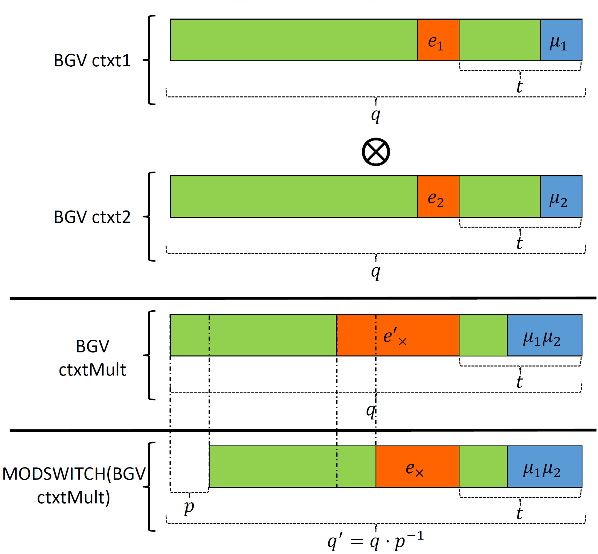
Figure 2: Ciphertext multiplication in BGV. Adapted from [CKKS17].
As shown in Figure 2, multiplication causes both components (payload) and noise to grow in magnitude. The multiplication result is contained within the space bounded by $t$, i.e., in the lower bits of the coefficient. The noise in the product grows similarly and takes some space from the noise budget. As mentioned previously, as long as the payload and noise are separate, decryption works successfully and the payload can be retrieved without errors. To obtain more intuition about the product ciphertext structure, let's work out the following algebraic equation: \begin{equation}\label{eq:bgv:mult:structure} \begin{split} \mu_1 \cdot \mu_2 + e'_{\times} &= (t e_1+\mu_1) \cdot (t e_2+\mu_2)\\ &= t^2 e_1 e_2 + t(e_1 \mu_2 + e_2 \mu_1) + \mu_1\mu_2 \end{split} \end{equation} To reduce the noise growth after multiplication, BGV includes a method called $\textsf{MODSWITCH}$ that takes as an input a ciphertext $\textsf{C}$ encrypting plaintext $\textsf{M}$ with coefficient modulus $q$ and returns an equivalent ciphertext $C'$ that encrypts the same plaintext but with a different coefficient modulus $q'$. Normally, $q' = \dfrac{q}{p}$ to reduce the noise, with $p$ being a number that divides $q$. Notice that this operation scales down the noise without affecting the payload component. The reason is that we choose $q'$ such that Equation \ref{eq:modswitch:constraint} is satisfied. In other words, from $t$'s perspective, $q$ and $q'$ are just the same. More concretely, we can work it out as shown in Equation \ref{eq:bgv:q:constraint}. \begin{equation}\label{eq:modswitch:constraint} q \equiv q' \mod t \end{equation} \begin{equation}\label{eq:bgv:q:constraint} \begin{split} q &\equiv q' \mod t \\ q &\equiv \frac{q}{p} \mod t \\ q &\equiv q \cdot p^{-1} \mod t \\ 1 &\equiv p^{-1} \mod t \end{split} \end{equation} From the above derivation, it is straightforward to see that multiplying by $p^{-1}$ is equivalent to multiplying by 1 modulo $t$. Therefore, the payload does not get affected by $\textsf{MODSWITCH}$ given that the constraint specified in Equation \ref{eq:modswitch:constraint} is satisfied. Note that after invoking $\textsf{MODSWITCH}$, the ciphertext moves from the level associated with $q$ to the next lower level associated with $q'$.
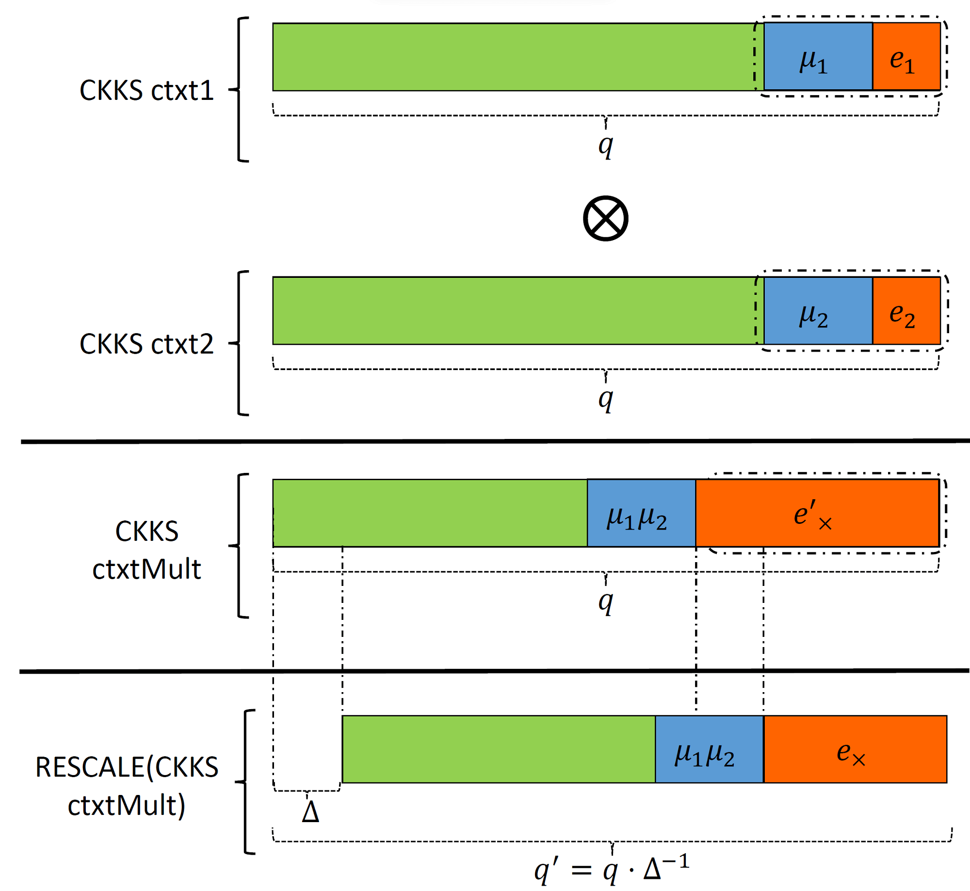
A slightly different behavior happens in CKKS. Figure 3 illustrates the inner working of CKKS homomorphic multiplication. The input plaintexts, each including payload and noise components merged as one chunk, are multiplied to generate the product of the payloads distorted by the multiplication error. We can work out Equation \ref{eq:ckks:mult:structure} similar to what we did in the BGV case. \begin{equation} \label{eq:ckks:mult:structure} \begin{split} \Delta^2 \mu_1 \cdot \mu_2 + e'_{\times} &= (\Delta \mu_1 + e_1) \cdot (\Delta \mu_2 + e_2)\\ &= \Delta^2 \mu_1 \mu_2 + \Delta(\mu_1 e_2 + \mu_2 e_1) + e_1e_2 \end{split} \end{equation} This is almost what we want except that the product payload is scaled by $\Delta^2$. To maintain the product at the same scale as the input, that is by $\Delta$, we can use $\textsf{MODSWITCH}$, which is called $\textsf{RESCALE}$ in CKKS terminology, to scale down the product by $\Delta$ and reduce the magnitude of multiplication noise. This step is similar to what we did in $\textsf{FPMul}$ \ref{eq:FPMul} to maintain the scale and precision fixed. Note that satisfying constraint \ref{eq:modswitch:constraint}, is no longer required for CKKS.
Figure 3: Ciphertext multiplication in CKKS. Adapted from [CKKS17].
10. Security of the Scheme
- Access for an encryption oracle: this means that Eve can choose a number of messages as she wishes and ask for encrypting them to generate valid corresponding ciphertexts. This is a very reasonable assumption since FHE can be deployed as a public-key encryption scheme, that is, the encryption key is publicly available and anyone can access it. Even if FHE is deployed in secret-key mode, this is still a reasonable assumption and it forms the basis of a commonly-known attack model INDistinguishability under Chosen Plaintext (IND-CPA).
- Ability to choose the function that would be evaluated homomorphically. This is also a reasonable assumption since Eve could be the server itself that is responsible for executing the outsourced homomorphic computation.
- Access to a decryption oracle: this means that Eve can choose a ciphertext and ask for its decryption. This is not a very far-fetched assumption as the decryption result might be shared after computation. Some applications might require the server to know certain decrypted values (to be provided in the clear by the client after decryption) to proceed with the application.
In response to this vulnerability, the attack proposers suggested tweaking the decryption function in CKKS by adding extra noise to the decryption result before publishing it to conceal the underlying RLWE noise. An open research problem is how to find tight bounds on the added noise such that CKKS is still secure under $\textsf{IND-CPA+}$ and the computational precision is not affected.
We remark that if the decryption result is never meant to be published or shared with untrusted parties, one can still use vanilla CKKS with no concerns about its security.
References
[APS15] Martin R Albrecht, Rachel Player, and Sam Scott. On the concrete hardness of learning with errors. Journal of Mathematical Cryptology, 9(3):169–203, 2015.
[BGV14] Zvika Brakerski, Craig Gentry, and Vinod Vaikuntanathan. (leveled) fully homomorphic encryption without bootstrapping. ACM Transactions on Computation Theory (TOCT), 6(3):1–36, 2014.
[CH18] Hao Chen and Kyoohyung Han. Homomorphic lower digits removal and improved fhe bootstrapping. In Annual International Conference on the Theory and Applications of Cryptographic Techniques, pages 315–337. Springer, 2018.
[CKKS17] Jung Hee Cheon, Andrey Kim, Miran Kim, and Yongsoo Song. Homomorphic encryption for arithmetic of approximate numbers. In International Conference on the Theory and Application of Cryptology and Information Security, pages 409–437. Springer, 2017.
[CSVW16] Anamaria Costache, Nigel P Smart, Srinivas Vivek, and Adrian Waller. Fixed-point arithmetic in she schemes. In International Conference on Selected Areas in Cryptography, pages 401–422. Springer, 2016.
[FV12] Junfeng Fan and Frederik Vercauteren. Somewhat practical fully homomorphic encryption. IACR Cryptol. ePrint Arch., 2012:144, 2012.
[HS15] Shai Halevi and Victor Shoup. Bootstrapping for helib. In Annual International conference on the theory and applications of cryptographic techniques, pages 641–670. Springer, 2015.
[LM21] Baiyu Li and Daniele Micciancio. On the security of homomorphic encryption on approximate numbers. In Annual International Conference on the Theory and Applications of Cryptographic Techniques, pages 648–677. Springer, 2021.
Appendices
A. Fixed-Point Arithmetic
It is crucial to understand that fixed-point numbers represented as integers have a scaling factor that is $(>1$ or $<1)$. For instance, if we used a fixed-point number represented as integer 17 associated with a scaling factor 1/10, then what we are actually referring to is 1.7.
A.1. Q Format
The dynamic range of a signed fixed-point format is bounded by $(a, a+2^{-f}, a+2^{-f}, \ldots, b-2^{-f}, b)$, where $a$ and $b$ are the minimum and maximum values supported by the format defined as follows: \begin{equation} \label{eq:Q:format:bounds} \begin{split} a &= -2^{m}\\ b &= 2^{m}-2^{-f} \end{split} \end{equation} Thus, in our $Q3.4$ format, the minimum supported number is $-2^{3} = -8$, and the maximum number is $2^{3}-2^{-4} = 8-2^{-4}$ = 7.9375, i.e., $Q3.4$ has the dynamic range $\{-8, -7.9375, \ldots, 7.9375\}$ with fixed step $2^{-4} = 0.0625$.
A.2. Arithmetic Operations
A.2.1 Conversions
To convert a real number $a$ with finite-precision to a $Qm.f$ fixed-point number,
simply multiply it with $2^f$ and truncate/round the fractional bits to integer.
The inverse conversion can be computed by dividing the fixed-point number by $2^f$.
\begin{equation} \label{eq:conv:real:to:fixed}
\begin{split}
\textsf{R2FP}(a) &= \textsf{RoundToInt or Truncate}(a\cdot2^f)\\
\textsf{FP2R}(a) &= \dfrac{a}{2^f}
\end{split}
\end{equation}
A.2.2 Addition and Subtraction
A.2.3 Multiplication and Division
We provide below an example of how to perform fixed-point arithmetic in $Q15.16$. The example was generated using $\texttt{C++}$. The real values of $a$ and $b$ are defined using the datatype $\texttt{float}$. The output precision was set to 9 using the command
cout.precision(std::numeric_limits<float>::max_digits10).
For each operation, we show 3 outputs;
- fixed-point result of the fixed-point operation,
- converted result from fixed-point to $\texttt{float}$
- the result as performed using IEEE-754 single-precision operations which can be used to serve as ground truth.
#include <iostream>
#include <math.h>
#include <limits>

using namespace std;

const int f = 16;
const int scaleFactor = (1 << f);
typedef std::numeric_limits<float> flt;

#define FloatToFixed(x) (x * (float)scaleFactor)
#define FixedToFloat(x) ((float)x / (float)scaleFactor)

#define Add(x, y) (x+y)
#define Sub(x, y) (x-y)
#define Mul(x,y) ((int64_t)((int64_t)x*y)/scaleFactor)
#define Div(x,y) ((int64_t)((int64_t)x*scaleFactor)/y)

int
main ()
{
    cout.precision(flt::max_digits10);

    float float_a = 1.3, float_b = 2.7;

    int fixed_a = FloatToFixed (float_a);
    int fixed_b = FloatToFixed (float_b);

    int fixedAdd = Add(fixed_a, fixed_b);
    int fixedSub = Sub(fixed_a, fixed_b);
    int fixedMul = Mul(fixed_a, fixed_b);
    int fixedDiv = Div(fixed_a, fixed_b);

    cout << "Output precision = " << flt::max_digits10 << " decimal digits\n";
    cout << "scale factor = (2^" << f << " = " << scaleFactor << ")" << endl << endl;
    cout << "a (float) = " << float_a << endl;
    cout << "b (float) = " << float_b << endl << endl;

    cout << "a (fixed): " << fixed_a << endl;
    cout << "b (fixed): " << fixed_b << endl;

    cout << "\nfixed add (fixed): " << fixedAdd << endl;
    cout << "fixed add (float): " << FixedToFloat(fixedAdd) << endl;
    cout << "float add (float): " << float_a+float_b << endl;

    cout << "\nfixed sub (fixed): " << fixedSub << endl;
    cout << "fixed sub (float): " << FixedToFloat(fixedSub) << endl;
    cout << "float sub (float): " << float_a-float_b << endl;

    cout << "\nfixed mul (fixed): " << fixedMul << endl;
    cout << "fixed mul (float): " << FixedToFloat(fixedMul) << endl;
    cout << "float mul (float): " << float_a*float_b << endl;

    cout << "\nfixed div (fixed): " << fixedDiv << endl;
    cout << "fixed div (float): " << FixedToFloat(fixedDiv) << endl;
    cout << "float div (float): " << float_a/float_b << endl;

    return 0;
}
Output precision = 9 decimal digits
scale factor = (2^16 = 65536)
a (float) = 1.29999995
b (float) = 2.70000005
a (fixed): 85196
b (fixed): 176947
fixed add (fixed): 262143
fixed add (float): 3.99998474
float add (float): 4
fixed sub (fixed): -91751
fixed sub (float): -1.40000916
float sub (float): -1.4000001
fixed mul (fixed): 230028
fixed mul (float): 3.50994873
float mul (float): 3.50999999
fixed div (fixed): 31554
fixed div (float): 0.48147583
float div (float): 0.481481463